What is a confusion matrix and how do I use binary classification metrics?

Confusion matrix cheat sheet pdf

I created an early version of the confusion matrix cheat sheet to keep at my desk as a quick reference for the definitions of machine learning classification metrics. Once I had it, I found it was useful in explaining model evaluation to business stakeholders and mentees in my work as a data scientist. I wanted to create a digital version to share with the data science community, and hopefully you find it as useful as I do.

Why this article?

This article explains the basic machine learning concepts behind the cheat sheet. It defines the related terms and serves as an entry point for readers less familiar with the ideas of binary classification in machine learning. This article also touches on how these ideas and techniques fit into the machine learning process in a business setting.

Overview

• What is a classification model
• Airport security: a motivating example
• What is a false positive, etc.?
• What is a confusion matrix?
• What are classification metrics?
  • Classification metrics list
• Classification considerations in the real world
  • Predicted probabilities
  • Binary metrics versus threshold-agnostic metrics and when to use each
  • Using multiple metrics (tradeoff pairs)
  • How to choose your metrics
  • Business simulation and cost-based threshold selection
  • Multiclass classification

What is a classification model?

Let’s start with some definitions:

• Classification model: a type of supervised predictive model that predicts what class (or group) a subject is a member of, where there are two or more mutually exclusive classes. Can be contrasted with regression models, which predict continuous numeric values.
• Prediction: a model’s educated guess about an unknown outcome. Classification models can make binary predictions (1,0) or probability predictions (decimal values between 1 and 0).
• Prediction threshold: a value between 0 and 1 used to convert probability predictions to binary ones. Observations with probability predictions greater than or equal to the threshold will be predicted positive (1) and those with probabilities lesser will be negative (0).
• Target: (aka label, actual, outcome): an outcome of interest or the record thereof. Target labels are used to train models that then predict the target when the outcome isn’t yet known. The term “actual” is used to distinguish a known outcome from a prediction made by a model on historical data (for evaluation purposes).
• Feature: a known attribute of a subject used to make a prediction. A model input.
• Class: One of the two-or-more categories that represent an attribute or event of interest. (e.g., on and off are both classes for the state of a light switch; yellow, red, and green are some possible classes for types of curries.) Classes are various possible values of classification targets.
• Categorical feature: Attributes of an observation that can be represented by two or more categories, such as (1,0) or (‘yellow’, ‘red’, ‘green’). Categorical features are inputs to the model, and as such are known attributes used to make predictions about an unknown outcome. Included here only to distinguish from classification target labels, which are categorical in nature, but which are the thing we attempt to predict. Other types of features could include continuous numeric, discrete numeric, ordinal, free text, images, sound, video, geospatial or other sensor data.
• Multiclass classification: a prediction paradigm in which the attribute of interest can take on more than two classes. Predicting eye color would be a multiclass problem.
• Binary classification: a type of prediction that involves sorting observations into two classes, often represented as 1 and 0.
• Positive class: (aka event, event of interest, occurrence): The event of interest in a binary classification problem. (e.g., for a model that predicts Hollywood hits, the event of interest would be producing a hit film, and thus that class would be represented by 1. For a model that predicts light switch position, the event of interest might be an observation of the switch made while the switch is on.)
• Negative class: the opposite of the positive class in a binary classification problem. Can be thought of as a default class, non-event or non-occurrence.
• Observation: a set of recorded measurements and characteristics of some subject at some point in time. Usually represented as a row in a dataset. A historical observation can include model features as well as the known outcome. A scoring observation’s outcome is unknown and the observation only includes features.
• Imbalance: the state of a data set having more outcomes of one class than the other(s). Usually the positive class is less prevalent than the negative in binary problems. This is because we usually consider a common class to be a default or non-event. We thus describe the rarer class as the “event” and label it with 1.
• Evaluation: measuring a model’s predictive power by using it to make predictions for observations with known outcomes and measuring how similar the predictions and actuals are.
• Evaluation metric: a statistic calculated to express a model’s predictive performance. Accuracy is one example of an evaluation metric.
• Scoring: either using a model to make predictions on unknown data or using model predictions made on historical data to calculate an evaluation metric for the model.
• Naive: a means of making predictions using only the available information about the target’s distribution in the training data. Naive binary predictions would always be the most common class in the training data. Naive probability predictions would always be the mean of the classes in the training data.
• Signal: the associations a model algorithm is able to discover that give it the ability to make predictions that are better than naive.
• Out-of-sample: the condition of an observation of having a known outcome but of having been held separate from the training data used to train a model. We use often want to use out-of-sample observations to evaluate a model in order to avoid the illusory effects of overfitting.
• Overfitting: the tendency of a predictive model to learn associations between features and outcomes that are random, but specific to the training data set, and thus do not generalize to the real world.

That will get us started, and we’ll define more terms as we go.

In machine learning, classification models are trained on historical data to make inferential predictions about the unknown class membership of a new observation.

We’ll focus primarily on binary classification and briefly touch on multiclass classification towards the end.

Airport security: a motivating example

Imagine we’re creating a classification model for use at an airport security checkpoint. We want to identify smugglers, so our binary classification target is 1 for smuggler and 0 for innocent traveler. The model might use the subject’s travel history or image data from an X-ray machine as feature inputs to make its predictions. For the purposes of this article, however, we’re going to ignore the model’s inputs and just focus on evaluating the quality of its predictions.

What is a False Positive, etc.?

To visualize this, let us represent our travelers as boxes. Smugglers have red dots and innocent travelers are empty boxes. The model circles the travelers it thinks are smugglers and ignores those it thinks are not.

From this, we can see that our model can be right in two ways and it can be wrong in two ways. These four prediction outcomes will populate the confusion matrix for our model:

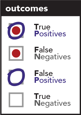
1. True Positive prediction (TP): accurately predicts when it sees evidence of contraband.
2. False Negative prediction (FN): falsely predicts that a traveler is innocent when they are, in fact, smuggling contraband.
3. False Positive prediction (FP): falsely predicts that a traveler is a smuggler when they’re really innocent.
4. True Negative prediction (TN): accurately predicts when a traveler is innocent.

Each of these types of predictions has three dimensions:

• the ability to be correct / incorrect
• the ability to represent a positive / negative prediction
• the ability to represent a positive / negative outcome

Note that of these dimensions, only the first two are made explicit in the names we use for each prediction outcome. For example, we know a False Positive prediction is a positive prediction that is wrong, but we must infer that the actual outcome was negative. This is annoying. In fact, that it’s a common joke that the confusion matrix got its name for being so confusing! The only piece of advice I can offer is to refer to the direction of the actuals as occurrences / non-occurrences or events / non-events to keep them distinguished from positive / negative predictions. If you have an alternative set of vocabulary, please share it!

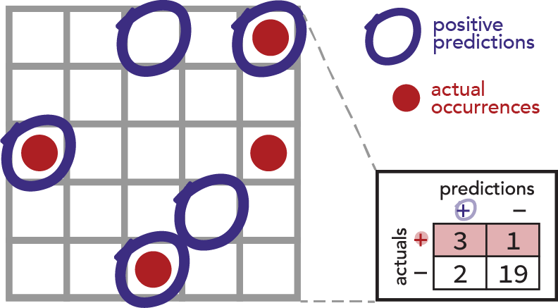
Back to our model. Imagine the model was trained on historical data where the actual guilt or innocence of travelers was determined by manual searches. Imagine we held out 25 of those observations from the model’s training data and set them aside as an out-of-sample validation set. This is important, of course, because we want to know how well our model generalizes to unseen travelers, not how closely fit it is to the original data. So we use our model to make predictions against the 25 validation rows and calculate our confusion matrix accordingly.

Each cell in the image above represents an observation of a traveler. Our model “circles” observations it thinks are positives. Actual positive occurrences (of smugglers) show up as red dots and non-occurrences (negatives) as empty cells.

What is a confusion matrix?

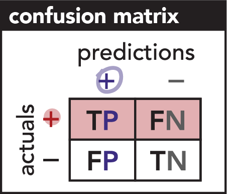
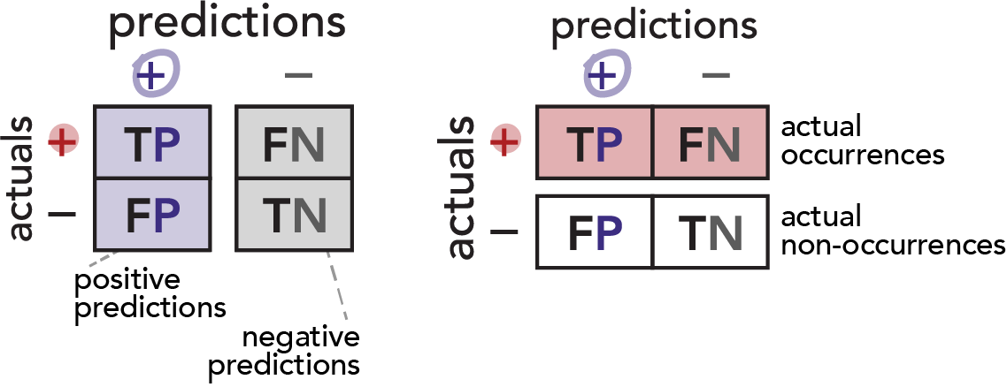
A confusion matrix is a grid that (at least for binary prediction) shows the counts of each the four prediction outcomes: True Positives, False Negatives, False Positives and True Negatives.

Here, our confusion matrix shows the positive / negative direction of our model’s predictions as two columns, and it shows the travelers’ actual status as two rows.

(Note that it would be just as valid to flip the axes of our confusion matrix–yielding columns that represent actuals and rows that represent predictions. Pay attention to axis labels on confusion matrices in the wild.)

It bears repeating: the name of a quadrant refers to the positive / negative direction of the model’s predictions and their correctness. The actual occurrence / non-occurrence of the event itself must be inferred. The key is to remember that “False Positives” is really referring to “falsely positive predictions” (and likewise with False Negatives).

What are classification metrics?

Seeing the counts in each quadrant can give us a vague sense of model performance, but we can do better.

To see how, consider a few questions we might want to answer about our airport security model:

• How accurate is this model? (What proportion of its predictions are correct?)
• How often would this model cause us to search innocent travelers?
• How often would this model allow smugglers to slip through security unnoticed?
• What proportion of searched travelers would actually be smugglers? (Answers at end of article)

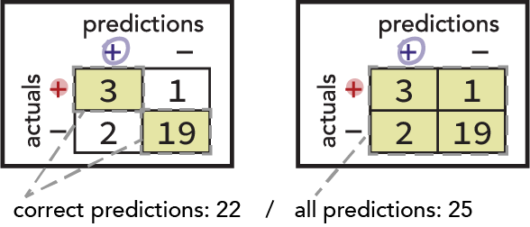
The most intuitive of these is the Accuracy question. You might already imagine dividing the number of correct predictions by the total number of observations. Here, that’s 22 / 25 = 0.88, or 88%. We can also express this ratio in terms of the confusion matrix quadrants: (TP + TN) / (TP + FN + FP + TN)

Next, consider the question about searching innocents. The relevant population is all innocent travelers. Notice that this is represented by the bottom row of our confusion matrix. The proportion of that population that our model falsely marks positive is of particular interest, and we therefore derive the False Positive Rate metric thusly: (FP) / (FP + TN)

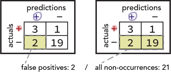
And so we can see that most of the classification metrics are rates / proportions constructed in a similar way. Except for Accuracy, they each use a row or column as a population of interest and describe how large one of its cells is as a proportion of it. Binary classification metrics are listed in the bottom left section of the cheat sheet and in the section to follow.

Returning to our example questions, think about the population relevant to the question about the proportion of smugglers that make it through the checkpoint. Can you find a relevant metric from the list below?

What about the proportion of searched travelers that are smugglers? Which count would you divide by which? Do you see a name for that metric in the list?

(Answers posted at the end of the article.)

Classification metrics list

These are the most-used of the binary classification metrics derived from the confusion matrix:

• Accuracy
  • the proportion of all predictions that are correct
  • appears high when dataset is imbalanced, even if model is no better than naïve (always predicts the majority class)
  • (True Positives + True Negatives) / (True Positives + False Negatives + False Positives + True Negatives)
• Precision / Positive Predictive Value
  • accuracy of positive predictions
  • proportion of searched w/ contraband
  • (True Positives) / (True Positives + False Positives)
• Recall / Sensitivity / True Positive Rate
  • proportion of actual occurrences correctly predicted positive
  • proportion of smugglers caught
  • (True Positives) / (True Positives + False Negatives)
• Specificity / True Negative Rate
  • proportion of non-occurrences correctly predicted negative
  • proportion of innocent travelers passed
  • (True Negatives) / (False Positives + True Negatives)
• False Positive Rate / False Alarm Rate
  • proportion of non-occurrences falsely predicted positive
  • proportion of innocent travelers searched
  • (False Positives) / (False Positives + True Negatives)
• False Negative Rate / Miss Rate
  • proportion of actual occurrences falsely predicted negative
  • proportion of smugglers passed
  • (false negatives) / (true positives + false negatives)
• F1 Score
  • harmonic mean of precision & recall
  • balances tradeoff between multiple metrics
  • assumes equal value/cost of true positives, false positives, true negatives and false negatives
  • 2 * ( [precision * recall] / [precision + recall] )

Note that with F1 Score, we assume that all quadrants of the confusion matrix are created equal. That’s not usually the case. For instance, we might say it’s worth $100 to catch a smuggler (the True Positive reward) but we only incur a $10 penalty if we search an innocent traveler (the False Positive cost).

(It’s useful to focus on True Positive reward and False Positive cost because the True Negative reward is usually 0 and the False Negative cost is usually 0 when comparing against an existing business practice. )

If we chose a model with the highest F1 Score, we might be too risk averse, searching too few people overall and letting pass more smugglers than optimal. There are other F-beta scores that weight the quadrants differently, and we could choose one of those.

An even better solution might be to treat our use case as an optimization problem where we solve for some quantitative value (such as dollars) instead of trying to maximize an arbitrary metric. We’ll discuss this in the section “Business simulation and cost-based threshold selection” below.

Classification considerations in the real world

Predicted probabilities

Most binary classification algorithms also allow for probability predictions, also known as raw scores. These are decimal values between 0 and 1 that seek to express the probability that an observation is an instance of the event of interest. This is useful because it gives some sense of how confident the model is, and it allows us to make our model more or less sensitive by changing our prediction threshold. But we’re suddenly faced with the problem of choosing a prediction threshold. The prediction threshold is the value above which we will consider a prediction to be positive and below which we’ll call it a negative.

For example, if the raw score for an observation row is 0.34, and our prediction threshold is 0.5, then that observation would be predicted negative (the score is below the threshold). If, however, we wanted to improve the Sensitivity of our model (which is the proportion of actual occurrences the model predicts positive), we may choose to decrease the threshold in order to make more of our predictions positive. Let’s say we change the threshold to 0.3. Now the observation with a raw score of 0.34 will be predicted positive.

Binary metrics versus threshold-agnostic metrics and when to use each

Because we can make probability predictions in addition to binary ones, we can also calculate evaluation metrics based on those probability predictions. I like to call these metrics threshold-agnostic; they quantify a model’s predictive performance (its ability to produce useful predictions) based on predicted probability, before we even think about choosing a prediction threshold.

Some examples of threshold-agnostic metrics:

• Area Under the ROC Curve (AUC): The proportion of the plotted area falling beneath the ROC (receiver operating characteristic) curve.
• Area Under the Precision-Recall Curve: The proportion of the plotted area falling beneath the Precision-Recall Curve. P-R AUC is usually a better choice for imbalanced problems than traditional AUC.
• Gini Norm: measures how well a model ranks observations. Great for problems that call for a sorted list of probabilities rather than binary predictions.
• Log Loss: measures the goodness-of-fit of predictions. Heavily penalizes overconfident, wrong predictions. Also good for imbalanced problems and those where proper calibration is important.

Threshold-agnostic metrics are particularly useful for helping us choose a modeling algorithm, features, and hyperparameters. We can then use binary classification metrics (like Precision and Recall) to help us choose a prediction threshold. We often do this by comparing tradeoffs in performance across multiple binary classification metrics over multiple thresholds and picking the threshold that yields the best result.

Using multiple metrics and how to choose (tradeoff pairs)

When we change the prediction threshold for a model, we see some classification metrics improve while others decline. A common technique is to pick two metrics that exhibit this tension and find a prediction threshold that strikes a balance between them.

Here are some examples of binary classification metric tradeoff pairs:

• Precision and Recall
• Sensitivity and Specificity
• True Positive Rate and False Positive Rate

Note that Recall is the same as Sensitivity and True Positive Rate! We call metrics by different names depending on how we pair them and the type of our use case.

Also note that True Positive Rate and False Positive Rate are the axes of the ROC curve, and that Precision and Recall are the axes of the P-R Curve.

How to choose your metrics

Precision and Recall both focus on True Positives and are useful when the True Positive reward is greater in magnitude than the False Positive cost. The Precision / Recall pair is well-suited to both balanced and imbalanced datasets.

Sensitivity and Specificity focus on correct predictions and are particularly useful when when both True Positives and True Negatives are important. This pair is also well-suited to imbalanced data. This is the go-to tradeoff pair for disease state tests such as covid tests.

True Positive Rate and False Positive Rate are suited to balanced datasets only. Use Precision and Recall for imbalanced datasets instead.

Note that several of the binary classification metrics are reciprocals of each other, meaning that they essentially provide the same information about a model and can be considered interchangeable.

Business simulation and cost-based threshold selection

If you can assign a set of costs and rewards to each of the prediction outcomes in your confusion matrix, then you can use simulation to select an optimal prediction threshold. I highly recommend this technique, as it ensures an optimal solution for your business team and comes with the silver lining of a dollars-per-year figure you can say your model (and data science team) contributes to your organization’s bottom line.

To do this, use out-of-sample predictions along with observed or assumed costs and rewards. If your costs and rewards are just a few aggregated figures that correspond the confusion matrix quadrants, then just multiply those values by the confusion matrix counts and sum them to calculate net profit (being sure to represent costs as negative numbers).

If your costs and rewards vary row by row, then you can sample from historical rows, make probability predictions, turn them into binary predictions at one threshold and then sum the rewards of the resulting True Positives and subtract from that the sum of the False Positive costs. (Typically, False Positive cost is not directly known and must be estimated or tested.) Rinse and repeat using a range of thresholds, and then simply pick the one that yields the greatest net profit.

Multiclass classification

Multiclass classification can be thought of as an extension of binary classification. In fact, you can make multiclass predictions using only binary models.

In One-versus-rest (OVR) modeling, one binary model is trained for every class, using all others as the negative class. In scoring, all models are used to predict the class, and the one with the highest predicted probability is the winner for that observation.

In One-versus-one (OVO) modeling, a binary model is trained for every possible combination of classes. This is impractical for multiclass problems with many classes, as the number of models required grows exponentially. At score time, all binary models make their predictions, and the “popular vote” (mode) of all binary models’ predictions becomes the multiclass prediction.

In addition, some modeling algorithms inherently support multiclass classification out of the box. These include many implementations of tree-based algorithms (decision trees, random forests, gradient boosting), K Nearest Neighbors and Naive Bayes models.

Answers (from “What are classification metrics?”):

• How accurate is this model? (What proportion of its predictions are correct?)
  • Accuracy
    • true predictions / all predictions
    • (True Positives + True Negatives) / (True Positives + False Negatives + False Positives + True Negatives)
• How often would this model cause us to search innocent travelers?
  • False Positive Rate
    • falsely positive predictions / all non-occurrences
    • False Positives / (False Positives + True Negatives)
• How often would this model allow smugglers to slip through security unnoticed?
  • False Negative Rate
    • falsely negative predictions / all actual occurrences
    • False Negatives / (False Negatives + True Positives)
• What proportion of searched travelers would actually be smugglers?
  • Precision / Positive Predictive Value
    • True Positives / all positive predictions
    • True Positives / (True Positives + False Positives)